Surface analyses with titanlib and gridpp
NOTE: Updated 2023-06-20 to reflect API changes in titanlib.
MET Norway produces gridded surface analyses every hour, which are used as input data to the current condtions on MET Norway’s weather site Yr (https://www.yr.no). These analyses are created by combining gridded output from a high resolution numerical weather prediction (NWP) model and observations from in-situ weather stations, using optimal interpolation (OI). Currently 2 m temperature and hourly precipitation are produced.

These analyses are produced using two open-source software packages developed at MET Norway. Titanlib is a quality control library that flags suspicious observations and gridpp is a post-processing library that, among other things, assimilates observations into gridded background fields from NWP models. Both packages are designed to support the operational use of large amounts of crowdsourced weather observations, such as personal weather stations from Netatmo, which is a rapidly growing source of weather information.
The libraries are written in C++, but they also have python interfaces (and in the future R interfaces). This post gives a step-by-step guide for creating surface analyses of temperature using titanlib and gridpp in python.
Getting started
First, install titanlib and gridpp python packages, which could be as easy as running the following commands:
pip3 install titanlib
pip3 install gridpp
… if you already have their non-python dependencies. If not, check out their respective webpages for installation instructions. You will also need to download the following four files:
| Type | Filename | Size |
|---|---|---|
| Observations | obs.nc | 9.3 KB |
| Ensemble background | analysis.nc | 110 MB |
| Output template | template.nc | 45 MB |
| Python code | surface_analysis.py | 4.3 KB |
The python code contains all of the code shown on this page and can be run to produce the figures below.
Quality control of observations
The first step is to ensure that only trustworthy observations are used, as erronerous observations can lead to large errors in the final analysis. For this we will use titanlib, but let’s start by reading observations and their station’s metadata from file into arrays:
import titanlib
import netCDF4
import numpy as np

with netCDF4.Dataset('obs.nc', 'r') as file:
    obs = file.variables['air_temperature_2m'][:, 0]
    obs_lats = file.variables['latitude'][:]
    obs_lons = file.variables['longitude'][:]
    obs_elevs = file.variables['altitude'][:]
    points = titanlib.Points(obs_lats, obs_lons, obs_elevs)
The obs variable now contains the observations [in Kelvin] in a 1-D arrays. obs_lats, obs_lons, and
obs_elevs are corresponding 1-D arrays of the stations’ latitudes [degrees], longitudes [degrees], and
elevations [m], respectively. These are used to create the points object, which is a tree-like structure that allows for
fast nearest neighbour lookup.
Spatial constistency test
Titanlib supports a variety of quality control methods, but we will focus on the spatial consistency test (SCT) here. The SCT compares each observations to what is expected given the other observations in the nearby area. If the deviation is large, the observation is removed.
The SCT has several parameters, which are described in detail on the titanlib
wiki. For a given observation, all other
observations within the outer_radius (in meters) will be used to compute a cross-validation value for the
observation. For computational efficiency, the cross-validation results will be reused for all observations
within the inner_radius such that the proceedure doesn’t have to be performed independently for every
observation. To further reduce computation time, only the num_max closest observations are used, even if
there are more than this many observations within the outer radius. The test is only performed if there are at
least num_min observations within the outer radius.
Let’s set up the parameters and run the test:
inner_radius = 50000
outer_radius = 100000
num_min = 5
num_max = 100
num_iterations = 1
num_min_prof = 20
dzmin = 100
dhmin = 10000
dz = 200
t2pos = np.full(len(obs), 4)
t2neg = np.full(len(obs), 4)
eps2 = np.full(len(obs), 0.5)

flags, sct, rep = titanlib.sct(points, obs,
        num_min, num_max, inner_radius, outer_radius, num_iterations,
        num_min_prof, dzmin, dhmin , dz, t2pos, t2neg, eps2)
The SCT function returns an array of flags with the same length as the input observations. A value of 0
denotes observations that passed the test and a value of 1 denotes those that are flagged. Let’s create
arrays that keep track of which observations are valid and invalid:
index_valid_obs = np.where(flags == 0)[0]
index_invalid_obs = np.where(flags != 0)[0]
Plotting the QC flags
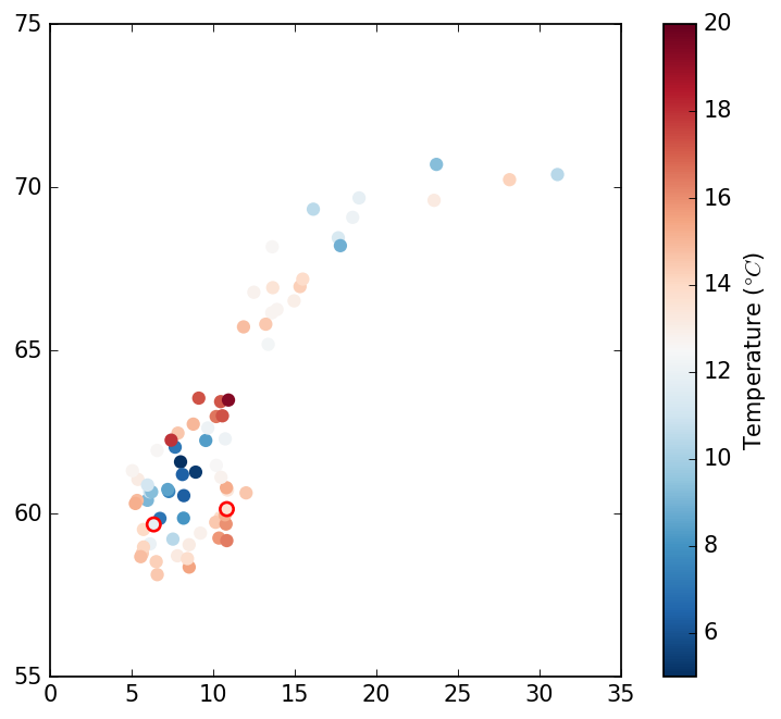
We can plot the observations, marking flagged ones with a black edge as follows:
import matplotlib.pylab as mpl
mpl.scatter(obs_lons[index_valid_obs], obs_lats[index_valid_obs],
        c=obs[index_valid_obs] - 273.15, s=50, linewidths=0, cmap="RdBu_r", vmin=5, vmax=20)
mpl.scatter(obs_lons[index_invalid_obs], obs_lats[index_invalid_obs],
        c=obs[index_invalid_obs] - 273.15, s=50, edgecolors="r", linewidths=1.5, cmap="RdBu_r",
        vmin=5, vmax=20)
mpl.xlim(0, 35)
mpl.ylim(55, 75)
mpl.gca().set_aspect(2)
cb = mpl.colorbar()
cb.set_label(r"Temperature ($\degree C$)")
mpl.show()
The SCT has identified two faulty observation in the southern part of the domain (shown by a red line surrounding the marker):

Creating the analysis
Once we have a set of trustworth observations, we can assimilate those into the NWP background. Gridpp provides a function that performs optimal interpolation (OI), which merges a background field and a set of observations, based on their relative accuracies.
Let’s start by reading in the data from the NWP data file, and the 1 km output template. We will first use the deterministic OI scheme, which takes a single ensemble member and for this we will take the control member, which has index 0 in the background file.
import gridpp
import numpy as np

with netCDF4.Dataset('analysis.nc', 'r') as file:
    index_control = 0
    blats_2500m = file.variables['latitude'][:]
    blons_2500m = file.variables['longitude'][:]
    belevs_2500m = file.variables['surface_geopotential'][0, 0, index_control, :, :] / 9.81
    bgrid_2500m = gridpp.Grid(blats_2500m, blons_2500m, belevs_2500m)
    background_2500m = file.variables['air_temperature_2m'][0, 0, index_control, :, :]

with netCDF4.Dataset('template.nc', 'r') as file:
    blats = file.variables['latitude'][:]
    blons = file.variables['longitude'][:]
    belevs = file.variables['altiude'][:]
    bgrid = gridpp.Grid(blats, blons, belevs)
bgrid_2500m and bgrid are objects that encapsulate the grid definitions.
Downscaling to 1 km
The background has 2.5 km grid spacing. To downscale to 1 km, we do a height correction. Operationally at MET Norway, we use a dynamic elevation gradient, but here we will use a constant -0.0065°C/m elevation gradient. Gridpp provides a method that does this downscaling, by taking the grid definitions, the original background field, and the desired elevation gradient as arguments:
gradient = -0.0065
background = gridpp.simple_gradient(bgrid_2500m, bgrid, background_2500m, gradient)
This yields a 1 km gridded field stored in background.
Observation operator
OI also requires the background values at the observation points, also called the observation operator. In many cases a simple method like nearest neighbour or bilinear is sufficient, however you could also compute the background in any otherway without gridpp. We will use gridpp’s bilinear interpolator:
points = gridpp.Points(obs_lats[index_valid_obs], obs_lons[index_valid_obs], obs_elevs[index_valid_obs])
pbackground = gridpp.bilinear(bgrid, points, background)
gridpp.Points creates an object that stores that encapsulates the point metadata (just like gridpp.Grid
does for a grid). pbackground is a vector with the model background at the observation points.
OI does not require you to specify the error variance of the background and the observations, only their ratios is needed. Since we trust observations more than the background, we set the ratio to 0.1:
variance_ratios = np.full(points.size(), 0.1)variance_ratios is a vector, one value for each observation, which means different observations can be
assigned different variance ratios if there is reason to believe that observations have different error
statistics.
Specifying the structure function
Optimal interpolation needs a structure function. We will use a Barnes function (Barnes 1973), with a horizontal decorrelation length of 100 km and a vertical decorrelation length of 200 m. This sets the limits to how far an observation will affect the adjustment of the background.
h = 100000
v = 200
structure = gridpp.BarnesStructure(h, v)
This structure function truncates the correlations past horizontal distances that are 3.64 greater than h.
Note, that this behvariour can be altered by specifing a different truncation distance hmax in the structure
function.
Currently, gridpp also supports a Cressman structure function, which uses a linear decorrelation function instead of an exponential. We aim to include further structure functions in the future.
Running the OI
When OI processes a gridpoint, it needs to invert a matrix containing all the observations within the
influence radius. In areas where the observation network is dense, this matrix can be come large and will
result in large computation times. However, in most cases reducing the number of observations doesn’t
negatively impact the accuracy of the analysis. We can set this using the max_points argument:
max_points = 50Note that this setting isn’t important in this example with only 75 observations, but when including Netatmo observations, this is critical.
Now we have defined all the required inputs and we can create a gridded analysis:
analysis = gridpp.optimal_interpolation(bgrid, background, points,
        obs[index_valid_obs], variance_ratios, pbackground, structure, max_points)
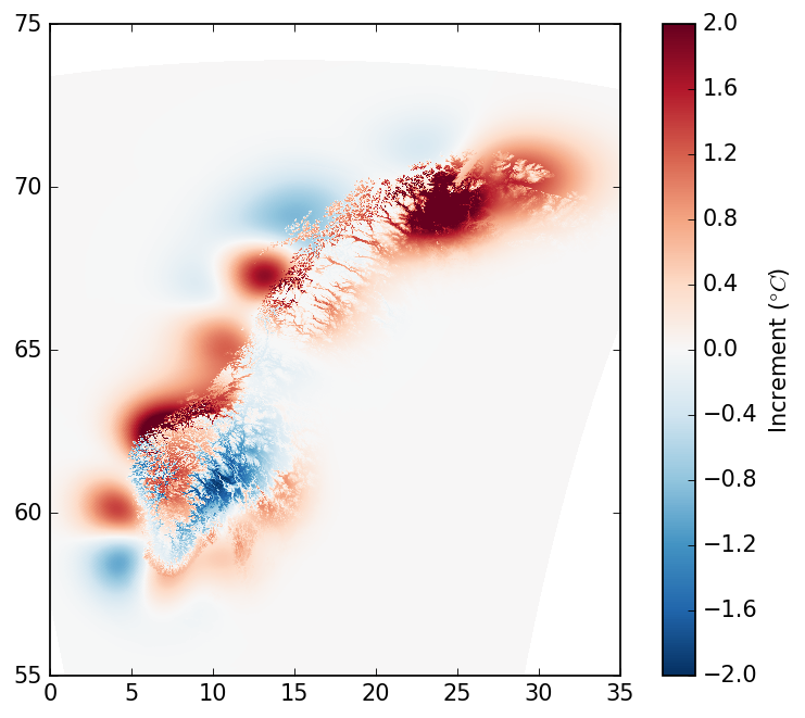
Plotting analysis increments
Finally, we can plot the analysis increments:
diff = analysis - background
mpl.pcolormesh(blons, blats, diff, cmap="RdBu_r", vmin=-2, vmax=2)
mpl.xlim(0, 35)
mpl.ylim(55, 75)
mpl.gca().set_aspect(2)
mpl.show()
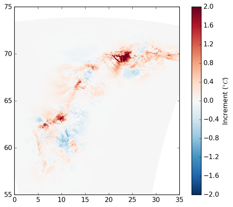
Ensemble mode
Gridpp also supports an Ensemble-based Statistical Interpolation (EnSI; Lussana et al. 2019) scheme that
uses spatial structure information from an ensemble of NWP model runs. This is the method used in the
operational temperature analyses used on Yr, as described by Nipen et al. 2020. To test this, you need to
load the full ensemble and ensure that the ensemble dimension is at the end. Also note that EnSI requires the
standard error of the observation (psigmas), which we set to 0.5°C. psigmas is a vector, one value for
each observation, which means different observations can be assigned different standard errors if there is
reason to believe that the observations have different error statistics.
with netCDF4.Dataset('analysis.nc', 'r') as file:
    background_ens_2500m = file.variables['air_temperature_2m'][0, 0, :, :, :]
    background_ens_2500m = np.moveaxis(background_ens_2500m, 0, 2)

num_members = background_ens_2500m.shape[2]
pbackground_ens = np.zeros([points.size(), num_members])
for e in range(num_members):
    background_ens = gridpp.simple_gradient(bgrid_2500m, bgrid, background_ens_2500m[:, :, e], gradient)
    pbackground_ens[:, e] = gridpp.bilinear(bgrid, points, background_ens)

psigmas = np.full(points.size(), 0.5)

analysis_ens = gridpp.optimal_interpolation_ensi(bgrid, background_ens, points,
        obs[index_valid_obs], psigmas, pbackground_ens, structure, max_points)
diff = (analysis_ens - background_ens)[:, :, index_control]
Further work
We have serveral features we want to implement. First of all, the OI presented here assumes Gaussian error characteristics. For non-Gaussian variables, such as wind and precipitation, we will support the transformation of the variable.
We also hope to support other structure functions. Gridpp can support structure functions that can provide a correlation function like this (in C++):
float corr(const Point& p1, const Point& p2)where p1 and p2 are points described by latitude, longitude, altitude, and land area fraction, and that
can use any arguments passed in the initialization of the class (such as h, v,hmax for BarnesStructure).
Finally, we plan to include an improvement to the EnSI scheme, which better handles variables such as precipitation, where the ensemble variance often is 0, when all members have no precipitation.
References
Barnes, S. L., 1973: Mesoscale objective map analysis using weighted time-series observations. NOAA Tech. Memo. ERL NSSL-62 [NTIS COM-73-10781], March, National Severe Storms Laboratory, Norman, Oklahoma, 60 pp.
Lussana, C, Seierstad, IA, Nipen, TN, Cantarello, L. Spatial interpolation of two‐metre temperature over Norway based on the combination of numerical weather prediction ensembles and in situ observations. Q J R Meteorol Soc. 2019; 145: 3626– 3643 (link)
Nipen, T.N., I.A. Seierstad, C. Lussana, J. Kristiansen, and Ø. Hov, 2020: Adopting Citizen Observations in Operational Weather Prediction. Bull. Amer. Meteor. Soc., 101, E43–E57 (link)